You're in a system design interview. The interviewer asks: Design WhatsApp for 2 billion users. How many messages per second should it handle?

No calculator. No Google. Just you, a pen, and paper.

Your mind goes blank. Two billion users sounds overwhelming.

But with back-of-the-envelope estimation, you can break this down in minutes using simple math.

This post shows you how to make quick, practical calculations that tell you if your system design will work or break under load.

What Is Back-of-the-Envelope Estimation?

Back of the envelope estimation is a quick way to make rough calculations that help you understand the scale, cost, or performance of a system before you build it.

You already use this kind of thinking in daily life. The name may feel new, but the idea is very simple.

Think of it like planning a party where you estimate:

• How many guests will come? (Users)

• How much food will each person need? (Data per user)

• How big should the venue be? (Server capacity)

The goal isn't to have perfect accuracy. It's getting numbers good enough to make smart decisions and avoid obvious disasters.

Where the Name Comes From

The phrase goes back to the late 1800s and early 1900s.

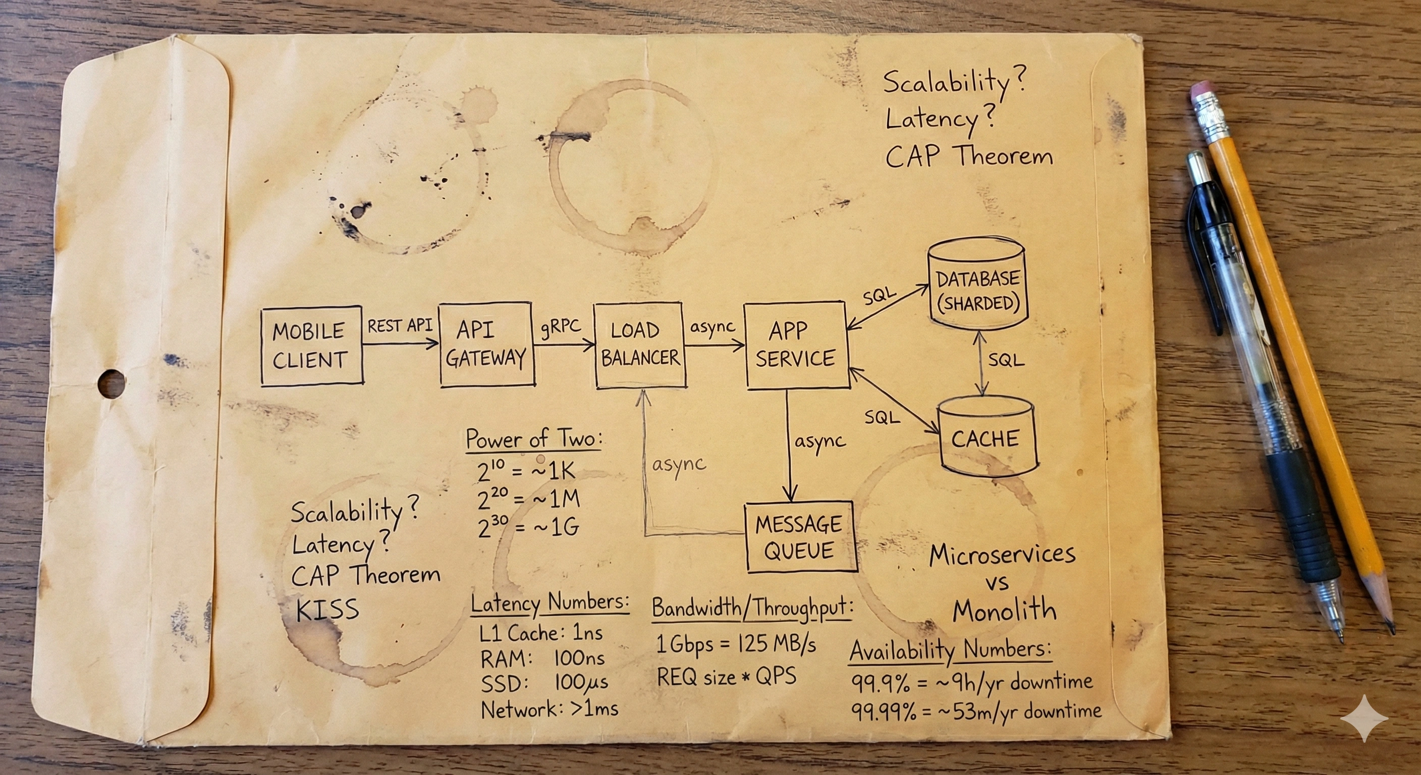
Scientists and engineers needed quick calculations on the spot. Envelopes were always nearby in offices and homes, and the blank backside made a convenient surface for rough math.

Einstein sketched ideas on spare paper. Enrico Fermi estimated the atomic bomb's power using simple math on whatever he had.

The phrase stuck because it captures the essence: quick, rough calculations using whatever's available.

Why This Matters for System Design

As an architect, you can't afford to guess. Every choice affects scale, cost, and reliability.

A few minutes of rough math tells you:

• Can your system handle peak traffic?

• Will your database keep up?

• Can your network support the load?

• Are your latency targets realistic?

• Will your cloud bill explode?

This skill helps you spot problems early, before writing a single line of code.

The best part? It's simple to learn.

Connect with the author on X and LinkedIn for insights on cloud architecture and system design.

The Building Blocks

To make quick estimations, you need to understand four fundamental concepts. Let's dive into each one.

Power of Two

When humans count, we naturally think in tens (10, 100, 1000..).

But computers don't count like we do. Everything in a computer uses bits and bit holds two states: 0 or 1, nothing else.

Because of this, computers count in powers of two, which is why it appears everywhere in computing.

Understanding this pattern makes size estimation much easier.

How Computers Count

At the smallest level, computers store information using bits. Each extra bit doubles the possible values you can represent.

2¹ = 2 possible values  
2² = 4 possible values  
2³ = 8 possible values  
2⁴ = 16 possible values  
2⁸ = 256 possible values

With 256 possibilities, you can represent a character, a color value, or a small piece of data. This is why 8 bits make 1 byte.

How Computers Measure Size

The same doubling pattern describes storage size:

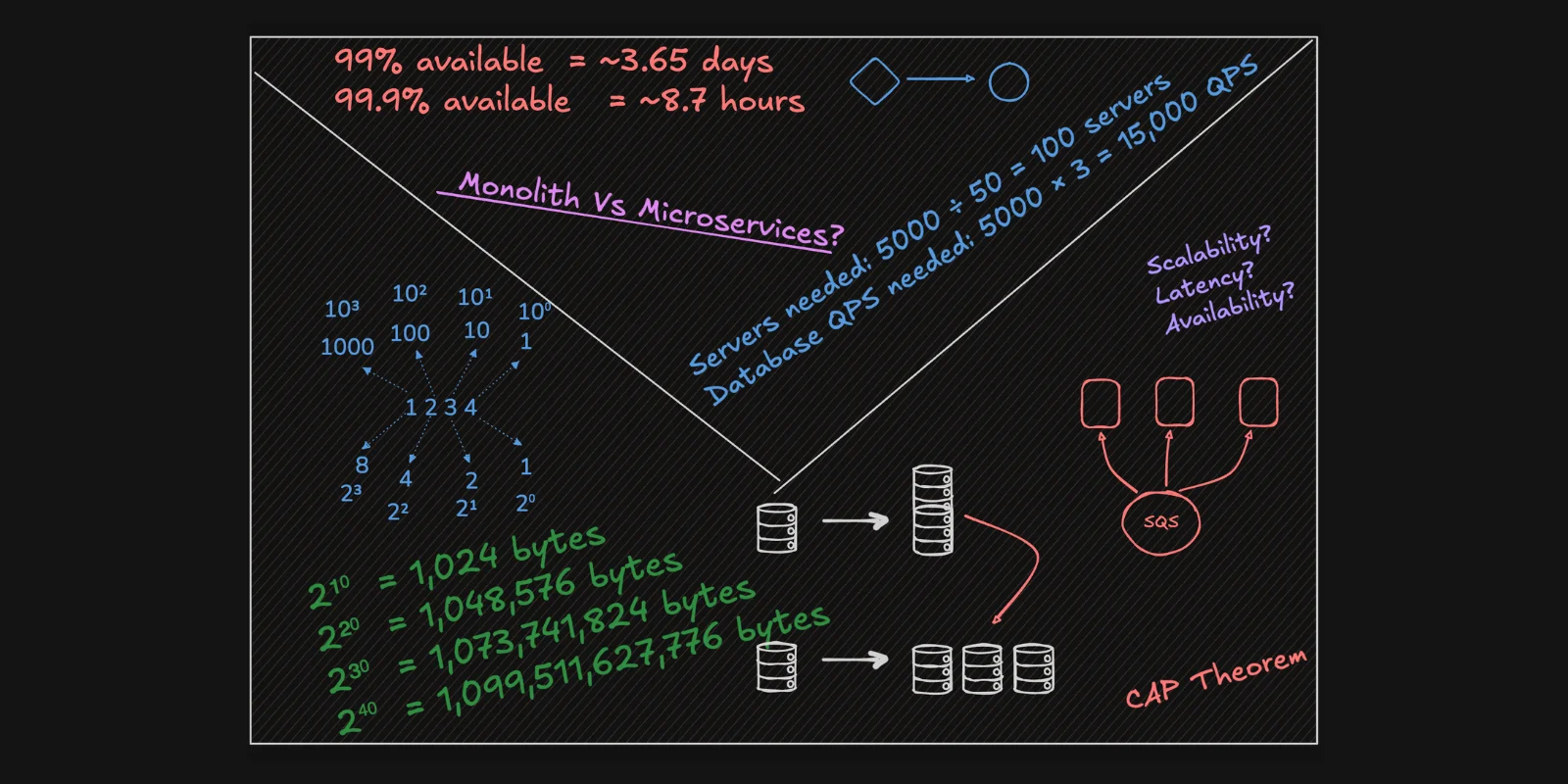
2¹⁰  = 1,024 bytes                → about one thousand bytes → 1 KB
2²⁰  = 1,048,576 bytes            → about one million bytes → 1 MB
2³⁰  = 1,073,741,824 bytes        → about one billion bytes → 1 GB
2⁴⁰  = 1,099,511,627,776 bytes    → about one trillion bytes → 1 TB
2⁵⁰  = 1,125,899,906,842,624 bytes → about one quadrillion bytes → 1 PB

These sizes power everything you estimate: storage, memory, bandwidth, cache, file sizes, and network limits.

The Key Pattern

• Bits describe how many different values something can represent.

• Bytes describe how much data something can hold or transfer.

Both follow powers of two.

Once this clicks, you start thinking like a computer, and estimation becomes natural.

Quick Examples

• A network moving 2 MB per second transfers about 2 million bytes every second.

• A cache with 64 MB holds about 64 million bytes of frequently accessed data.

• A 4 MB image contains about 4 million bytes of pixel information.

These mental shortcuts let you reason about size without calculators.

Latency Numbers

Latency is how long something takes to respond.

In a system, that “something” could be a CPU operation, a memory read, a disk access, or a network request. Each takes a different amount of time and some are extremely faster than others.

Once you understand what’s fast and what’s slow, it becomes much easier to see where your design might fall apart.

Units of Time

nanosecond (ns) < microsecond (µs) < millisecond (ms) < second

1 second = 1,000 milliseconds
1 millisecond = 1,000 microseconds  
1 microsecond = 1,000 nanoseconds

This scale shows just how big the speed gaps are inside a computer.

How Fast Are Different Operations?

Here is a simple version of real latency numbers:

L1 cache read              → ~0.5 ns   (basically instant)
CPU operation              → ~1 ns
Memory read                → ~100 ns
Same-region network call   → ~500 µs
Disk read                  → ~10 ms
Cross-continent network    → ~150 ms

You don't need to memorize exact values. What matters is the pattern.

The Pattern That Matters

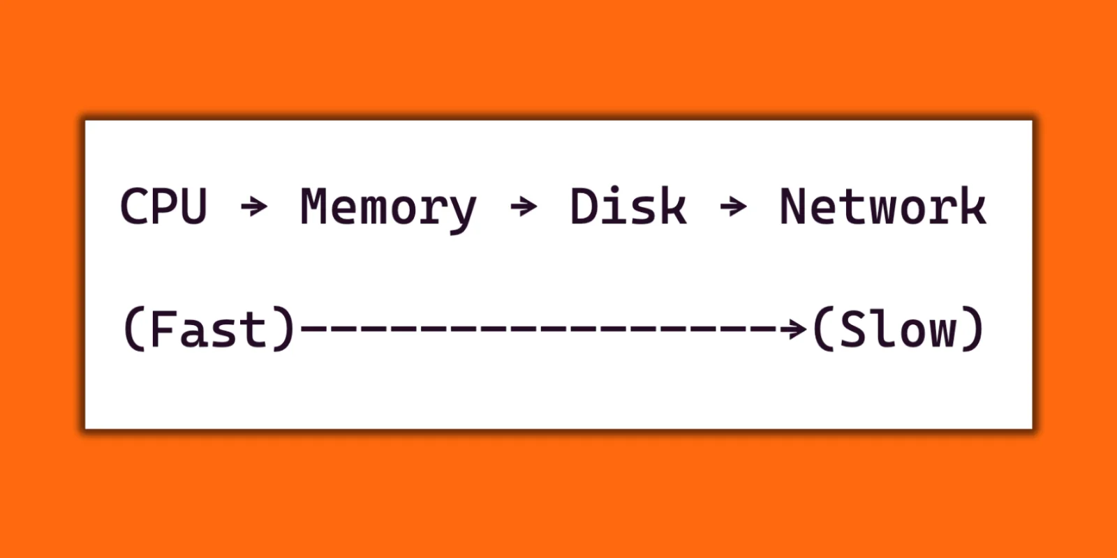
• CPU is thousands of times faster than memory

• Memory is hundreds of times faster than disk

• Disk is much faster than network

• And global network calls are the slowest of all

This simple pattern explains why caching works, why databases become bottlenecks, and why smart architecture tries to keep everything as close and local as possible.

Real Design Decisions

Example 1: Understanding Request Speed

Suppose a user request (like loading a profile page) makes three database calls. Each database call takes 5 ms.

• 3 DB calls → 15 ms

• App logic → 5 ms

• Total → 20 ms per request

If one request takes 20 ms, a single server can handle: 1 second / 0.020 = ~50 requests per second (RPS)

But here's the key insight. Each request makes 3 database calls, so: 50 RPS × 3 DB calls = 150 queries per second (QPS) to the database.

Now you can see two potential bottlenecks:

• Server capacity: 50 RPS

• Database capacity: 150 QPS

If your app expects 5000 concurrent user requests, you need:

• Servers needed: 5000 ÷ 50 = 100 servers

• Database QPS needed: 5000 × 3 = 15,000 QPS

This is back-of-the-envelope estimation in action. In two minutes, you know your system needs 100 servers and a database that can handle 15,000 queries per second.

Example 2: Why Caching Works

Since memory (100 ns) is hundreds of times faster than disk (10 ms), certain questions become obvious:

• Can I cache this instead of hitting the database every time?

• Can I pre-compute this instead of recalculating it on every request?

Before understanding latency, these seemed like random optimizations. Now they're natural design choices based on speed differences.

Bandwidth and Throughput

Bandwidth and throughput both describe how much data moves through your network, but they measure different things.

Bandwidth = your network's maximum capacity(like pipe width). It's the theoretical limit of how much data can flow.

Throughput = is the actual, real-world rate of data transfer (what you actually get). It's usually less than bandwidth due to congestion, packet loss, or other real-world factors.

Real example:

Your internet plan might offer 100 Mbps bandwidth, but during peak hours you might only get 70 Mbps throughput because everyone in your area is streaming video.

Understanding the Units

When you buy internet, companies advertise 100 Mbps speed! But when you download a file, your computer shows 12 MB/s. This isn't misleading, they're measuring differently.

Networks are measured in bits per second because that's how data travels through cables and routers. Every piece of network equipment thinks in bits.

But your computer shows file downloads in bytes per second because that's how we measure file sizes. A photo is 2 MB, so downloads naturally show in the same units.

The conversion: 1 byte = 8 bits

This means:

8 Mbps internet = 1 MB/s maximum download speed
80 Mbps internet = 10 MB/s maximum download speed  
800 Mbps internet = 100 MB/s maximum download speed

For system design, remember this conversion. If you need to transfer 100 MB/s of data, you actually need 800 Mbps of network capacity.

Common Network Speeds

Here are typical bandwidth numbers you'll encounter when designing systems:

Home internet:     100 Mbps  (12 MB/s maximum transfer)
Office internet:   1 Gbps    (125 MB/s maximum transfer)
Server connection: 10 Gbps   (1.25 GB/s maximum transfer)
CDN backbone:      100 Gbps  (12.5 GB/s maximum transfer)

These numbers help you understand what's realistic for different connection types. A home user uploading a video will be limited by their 12 MB/s connection, while your servers can handle much higher loads.

Real Design Examples

Example 1: Photo Upload Service

You're building an app where users upload 10 MB photos. You expect 1000 uploads per hour during peak time.

Let's calculate the bandwidth needed:

Total data per hour: 1000 photos × 10 MB = 10,000 MB = 10 GB/hour
Data per second: 10 GB ÷ 3600 seconds = 0.00278 GB/s
Convert to MB/s: 0.00278 × 1000 = 2.78 MB/s ≈ 3 MB/s
Convert to Mbps: 3 MB/s × 8 = 24 Mbps

Example 2: Video Streaming Platform

You have 10,000 users simultaneously streaming 1080p video at 4 Mbps each during prime time.

Total bandwidth needed: 10,000 users × 4 Mbps = 40 Gbps

A single server with a 10 Gbps connection can't handle this load. You need either 4 servers or a Content Delivery Network (CDN) to distribute the load across multiple locations.

How Bandwidth and Throughput Work Together

Bandwidth and throughput are connected, but they tell different stories about your network performance.

Your server might have 10 Gbps bandwidth, but the actual data flowing through it right now could be much less.

• Throughput can never exceed bandwidth, but it's almost always lower.

• The gap between them tells you about network health

In a healthy network, you typically see throughput reaching 70-90% of your total bandwidth. The remaining 10-30% gets consumed by network overhead, protocol headers, and minor congestion. This is completely normal.

When throughput drops significantly below bandwidth, something is wrong.

Availability Numbers

Availability measures how often a system is actually working.

It tells you how much of the time your service is up and usable. Usually, it is written as a percentage, and people often describe it using the word nines.

For example: 99%, 99.9%, 99.99%.. and so on.

At first glance, these numbers look almost the same. But in reality, each extra nine makes a big difference in how much downtime is allowed.

What the Numbers Mean

Here's what different availability levels mean over one year:

99% available     = ~3.65 days of downtime per year
99.9% available   = ~8.7 hours of downtime per year
99.99% available  = ~52 minutes of downtime per year
99.999% available = ~5 minutes of downtime per year

When you see it like this, the gap becomes very clear.

Going from 99.9 to 99.99 can remove entire hours of possible downtime. And each extra nine becomes harder and more expensive to achieve.

The Math Behind It

Availability is simple to calculate:

Availability (%) = (Total Time - Downtime) / Total Time × 100

Example: A year has 8,760 hours. If your app was down for 48 hours in that year:

• Availability = (8,760 - 48) ÷ 8,760 × 100 = 99.45%

The availability numbers you see aren't guesses. They come from real measurements of uptime and downtime.

Why This Matters for Design

Availability directly influences your architecture before you write any code.

As an architect, one of the most important questions you need to ask is how much downtime is acceptable for the application. That is usually a business decision, not a technical one.

If the business can handle a few days of downtime in a year, then a simple setup might be enough. A single server and a single database could work.

But if the business can only tolerate a few minutes of downtime, then the design must be very different. You will need multiple servers, replicas, automatic failover, load balancing, and maybe even multiple regions.

In that way, availability directly influences your architecture, your cost, and your overall complexity before you even start building.

And once the system is live, availability also helps you understand how healthy it really is.

You can calculate it monthly, quarterly, or yearly to track trends, see where problems are happening, and improve over time.

Putting It All Together

Now you understand the four building blocks:

• Power of Two for storage calculations

• Latency for performance and capacity planning

• Bandwidth and Throughput for network capacity

• Availability for reliability requirements

Let's see how they work together in a real example.

Complete Example: Designing a Photo Sharing App

Requirements:

• 10 million daily active users

• Each user uploads 2 photos per day

• Each photo is 2 MB

• Users view 20 photos per day

• Target: 99.9% availability

Storage Estimation (Power of Two):

Daily uploads: 10M users × 2 photos = 20M photos/day
Daily storage: 20M photos × 2 MB = 40M MB = 40 TB/day
Yearly storage: 40 TB × 365 = 14,600 TB ≈ 15 PB/year

Traffic Estimation (Latency):

Daily requests: 10M users × 20 photo views = 200M requests/day
Requests per second: 200M ÷ 86,400 seconds ≈ 2,315 RPS
Peak traffic (3x average): ~7,000 RPS

Bandwidth Estimation (Bandwidth & Throughput):

Upload bandwidth:
- 20M photos/day × 2 MB = 40 TB/day
- 40 TB ÷ 86,400 seconds ≈ 463 MB/s
- Convert to Mbps: 463 × 8 ≈ 3,700 Mbps ≈ 4 Gbps

Download bandwidth:
- 200M views/day × 2 MB = 400 TB/day
- 400 TB ÷ 86,400 seconds ≈ 4,630 MB/s ≈ 37 Gbps
- Peak (3x): ~111 Gbps

Add 30% buffer for real throughput: ~145 Gbps needed

Availability Planning:

99.9% availability = 8.7 hours downtime/year allowed
This requires:
- Load balancers
- Multiple servers
- Database replication
- Automated failover
- Monitoring and alerts

Quick Decisions You Can Make:

• Need CDN for photo delivery (111 Gbps peak is too much for single location)

• Need object storage like S3 (15 PB/year is massive)

• Need caching layer (memory is 100x faster than disk for popular photos)

• Need multiple regions for availability target

• Database will handle 2,315 QPS average, 7,000 QPS peak

All of this from 10 minutes of back-of-the-envelope math.

Final Thoughts

With these four building blocks, you can:

• Estimate if your design will work before building it

• Spot bottlenecks early

• Make informed architecture choices

• Communicate clearly with stakeholders

• Avoid expensive mistakes

Remember two key things:

First, these methods give you rough estimates, not exact numbers. Always add a 20-50% buffer to whatever you calculate. This handles unexpected traffic spikes and real-world conditions.

Second, the more you practice, the more natural it becomes. Start with simple examples. Work through system design problems. Soon you'll be doing these calculations in your head.

I hope this guide has provided you valuable information.

If you enjoyed this article, feel free to connect with me through my Linktree 🌳, where you'll find all my social links.

Thanks for reading.

– Alon